Finding Highly Correlated Features

Table of Contents

1. Motivation
2. Implementation
3. Parameterisation

Motivation

From a modelling perspective, it is not a big problem to have highly correlated features in the dataset. We have regularised Lasso/Ridge regression that are designed to deal with this kind of dataset. The ensemble trees are robust enough to be almost immune from this. Of course all model requires proper hyperparameter tuning with proper cross validation.

The problem raises in understanding the feature contributions: if there are 5 features that are highly correlated, and their individual contribute could be tiny, but their true contribution should be aggregated by adding the contribution together and considered them as a group, e.g. adding their coefficients in Ridge, and adding feature importance in LightGBM.

If their aggregated feature importance turns out to be indeed little, I can remove them from the model to have a simpler model. A mistake I used to make is removing the correlated features based on their individual feature importance, it leads to less performant models.

A better and cleaner approach is to the clean up correlated features to begin with, then I won’t need to do the feature importance aggregation, and it would speed up the model development cycle: there are less features to look at, to train the model, to verify the data qualities etc. When the model goes live in production, it translates to less data to source and maintenance.

Implementation

So I need to enrich my tool set to identify highly correlated features. I couldn’t find an existing library that does that, so I implemented it myself.

The key steps are:

1. Based on the correlation matrix, create a correlation long table. Each row stands for the correlation between feature $X_1$ and feature $X_2$. Assuming there are three features in the dataset, the table looks like this.

   Row	X1	X2	Corr
   1	A	B	0.99
   2	A	C	0.80
   3	B	C	0.95

2. Remove rows if the correlation is less than the threshold $T$. It significantly reduces the input to Step 3.

   If the threshold is 0.9, then the Row 2 will be removed.

3. Treat the correlation table as a directed graph,

   1. Let $E$ be the unexplored nodes, filled with all the features $X_1$ in the start, $R$ is the result.

   2. For each node in $E$,

      1. Continue to travel the graph in depth-first fashion until there is no connections left, and add the connected node to the result $R$ at each visit.

      2. Remove the connected nodes in $R$ from the remaining nodes to explore in $E$.

The vanilla Python code corresponding to Step 3 is listed below. The ds object is a pandas.DataFrame, multi-indexed by $X_1$ and $X_2$, so ds.loc['A'].index gives all the connected features from $A$ whose correlation with $A$ is large than the provided threshold.

 
def find_neighbors(ds: pd.DataFrame, root: str, res: set):
    """recursively find the nodes connected with root in graph ds.
    """
    res.add(root)
    if root in ds.index:
        ns = ds.loc[root].index.tolist()
        for n in ns:
            find_neiboughr(ds, n, res)
    else:
        return []

def find_correlated_groups(ds: pd.DataFrame):
    """
    The ds object is a pandas.DataFrame, multi-indexed by X1 and X2.
    """
    res = defaultdict(set)

    # contiune til all nodes are visited.
    cols = ds.index.get_level_values(0).unique().tolist()
    while len(cols) != 0:

        # always start from the root as ds is directed graph.
        col = cols[0]
        find_neighbors(ds, col, res[col])

        # remove connected nodes from the remaining.
        for x in res[col]:
            if x in cols:
                cols.remove(x)
    return res

The result is a collection of mutually exclusive groups. Each group contains a set of highly correlated features, for example

The next step is to decide which feature to keep and remove the rest within each group. The deciding factors can be data availability (e.g. choose the one feature with less missingness), costs in data sourcing (e.g. free to download from the internet) or familiarity (e.g. the feature is well understood by people) etc.

Parameterisation

There are two hyperparameters:

• The correlation type: It can be Pearson for numerical data and Spearman for ordinal/categorical data. For a large dataset, it would take some time to calculate the correlation matrix.

• The correlation threshold $T$: The higher the threshold, the less number of features to remove, so it is less effective. However, if the threshold is set too low, it leads to a high false positive rate, e.g. two features can be correlated, but they can still complement each other in the model.

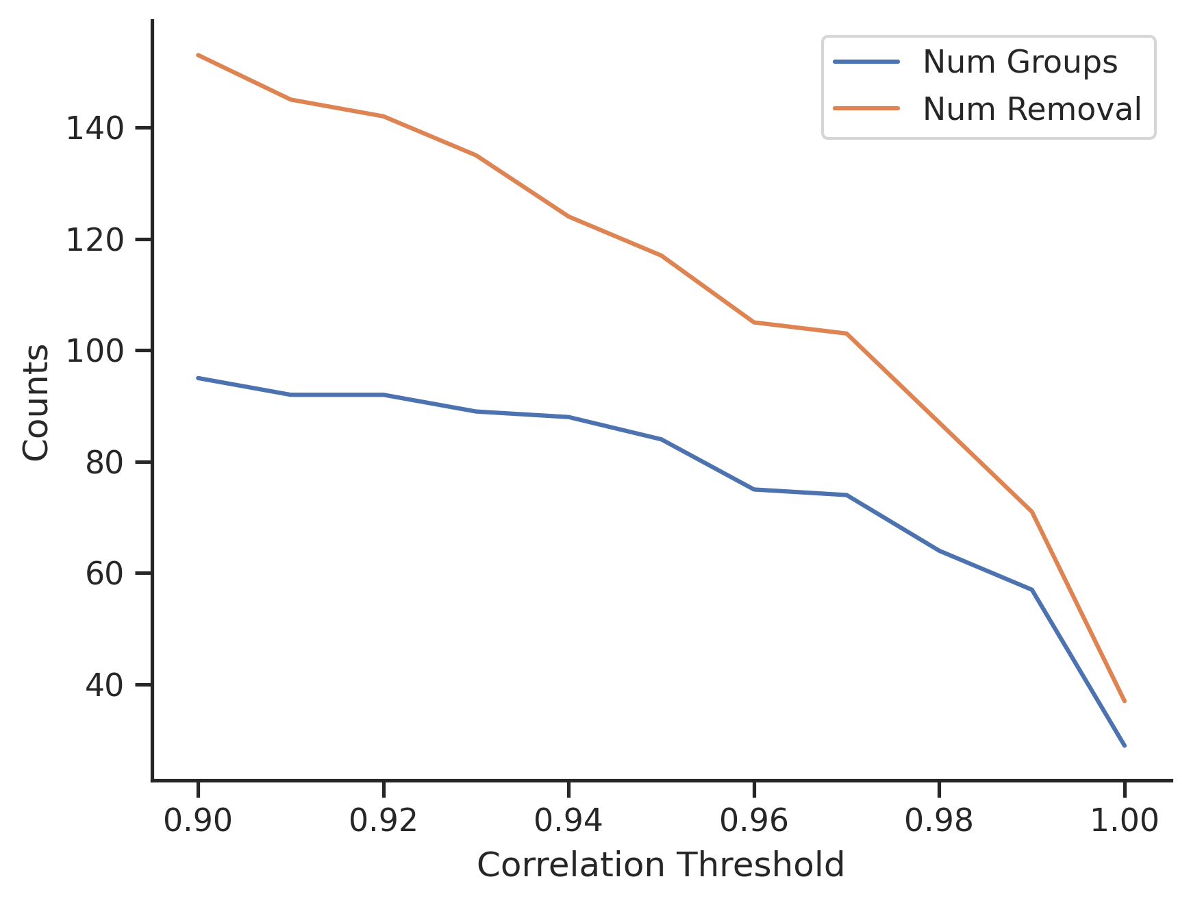
I would test a range of values from 0.9 to 1, and review the results. Below graph shows the number of features to remove with varying thresholds.

• When $T=0.9$, there are about 95 groups, and in total 153 features to remove.
• When $T=1$, there are 29 groups, and in total 37 features to remove.

Proper end-to-end test runs are required to identify the best hyperparameters. As a quick rule of thumb, those 37 duplicated features identified with $T=1$ can be dropped without further testing.

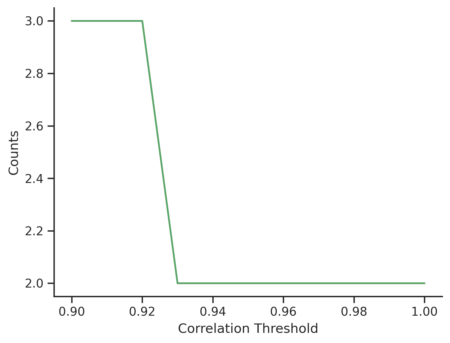
The group sizes with varying thresholds $T$ provide an interesting insight of the data. The 75% percentile of the group sizes is plotted, which suggests that apart from the 33 duplicated features, there are a large number of paired features (i.e. group size is 2) whose correlation is large, more than 92%.